After tokenization, we have sequences of integer IDs. But a neural network can't learn from raw integers - we need dense vector representations that capture semantic meaning. This is where embeddings come in.
- The Problem: Numbers Without Meaning
- What Are Embeddings?
- The Embedding Lookup
- Numeric Example
- Why Embeddings Work
- Embedding Dimensions
- Code Implementation
- Visualization
- Training Embeddings
- References
After tokenization, we have:
"The cat sat" → [42, 156, 89]
But these numbers are arbitrary! Token 156 ("cat") isn't mathematically closer to token 157 ("dog") than to token 2500 ("quantum"). The integer IDs carry no semantic information.
If we fed raw token IDs directly to a neural network:
# BAD: Raw IDs as input
input = [42, 156, 89]  # "The cat sat"

# Problems:
# 1. "cat" (156) seems "closer" to "car" (155) than "kitten" (3421)
# 2. Model can't generalize: knowing about "cat" doesn't help with "dog"
# 3. Scale varies wildly (ID 1 vs ID 50000)An embedding is a learned lookup table that maps each discrete token ID to a continuous vector of numbers.
Token ID 156 ("cat")  →  [0.12, -0.34, 0.87, 0.05, ..., -0.23]
                          ↑                                  ↑
                          |______ embedding_dim values ______|
- Dense: Unlike one-hot encoding, embeddings use fewer dimensions but all values are non-zero
- Learned: Values are optimized during training, not hand-crafted
- Semantic: Similar words naturally cluster together in the vector space
| Representation | "cat" with vocab_size=5000 |
|---|---|
| One-Hot | [0,0,0,...,1,...,0,0,0] (5000 dims, mostly zeros) |
| Embedding | [0.12, -0.34, 0.87, ...] (128 dims, all informative) |
The embedding layer is simply a matrix of shape (vocab_size, embedding_dim):
Embedding Table E (vocab_size × embedding_dim):
         ┌─────────────────────────────────┐
Token 0  │  0.02  -0.15   0.33  ...  0.04  │ ← embedding for "<PAD>"
Token 1  │ -0.11   0.45   0.12  ...  0.78  │ ← embedding for "<UNK>"
Token 2  │  0.85  -0.22   0.67  ... -0.31  │ ← embedding for "the"
   ...   │  ...    ...    ...   ...   ...  │
Token 156│  0.12  -0.34   0.87  ... -0.23  │ ← embedding for "cat"
   ...   │  ...    ...    ...   ...   ...  │
Token N  │ -0.45   0.08   0.19  ...  0.56  │
         └─────────────────────────────────┘
              e₀     e₁     e₂   ...  e_d
Lookup operation: Given token ID i, return row E[i]
Let's work through a concrete example:
Vocabulary size: 5 tokens
Embedding dimension: 4

Embedding Table E (5 × 4):
         ┌─────────────────────────┐
Token 0  │  0.1   0.2   0.3   0.4  │  "a"
Token 1  │  0.5   0.6   0.7   0.8  │  "cat"
Token 2  │  0.9   1.0   1.1   1.2  │  "sat"
Token 3  │  1.3   1.4   1.5   1.6  │  "on"
Token 4  │  1.7   1.8   1.9   2.0  │  "mat"
         └─────────────────────────┘
Text: "a cat sat"
Token IDs: [0, 1, 2]
# For each token ID, look up its row in E
token_0 = E[0] = [0.1, 0.2, 0.3, 0.4]  # "a"
token_1 = E[1] = [0.5, 0.6, 0.7, 0.8]  # "cat"
token_2 = E[2] = [0.9, 1.0, 1.1, 1.2]  # "sat"

# Stack into a matrix
embeddings = [[0.1, 0.2, 0.3, 0.4],    # Position 0: "a"
              [0.5, 0.6, 0.7, 0.8],    # Position 1: "cat"
              [0.9, 1.0, 1.1, 1.2]]    # Position 2: "sat"

# Shape: (sequence_length, embedding_dim) = (3, 4)With multiple sequences:
# Batch of 2 sequences, each length 3
batch_token_ids = [[0, 1, 2],   # "a cat sat"
                   [1, 2, 4]]   # "cat sat mat"

# After embedding lookup
batch_embeddings = [
    # Sequence 1: "a cat sat"
    [[0.1, 0.2, 0.3, 0.4],
     [0.5, 0.6, 0.7, 0.8],
     [0.9, 1.0, 1.1, 1.2]],

    # Sequence 2: "cat sat mat"
    [[0.5, 0.6, 0.7, 0.8],
     [0.9, 1.0, 1.1, 1.2],
     [1.7, 1.8, 1.9, 2.0]]
]

# Shape: (batch_size, sequence_length, embedding_dim) = (2, 3, 4)After training, embeddings capture semantic relationships:
                    Embedding Space (2D visualization)
                              ↑
          "queen" ●          │
                             │         ● "woman"
                             │
       "king" ●              │              ● "man"
                             │
  ─────────────────────────────────────────────────→
                             │
             "dog" ●         │          ● "cat"
                             │
                  "puppy" ●  │    ● "kitten"
                             │
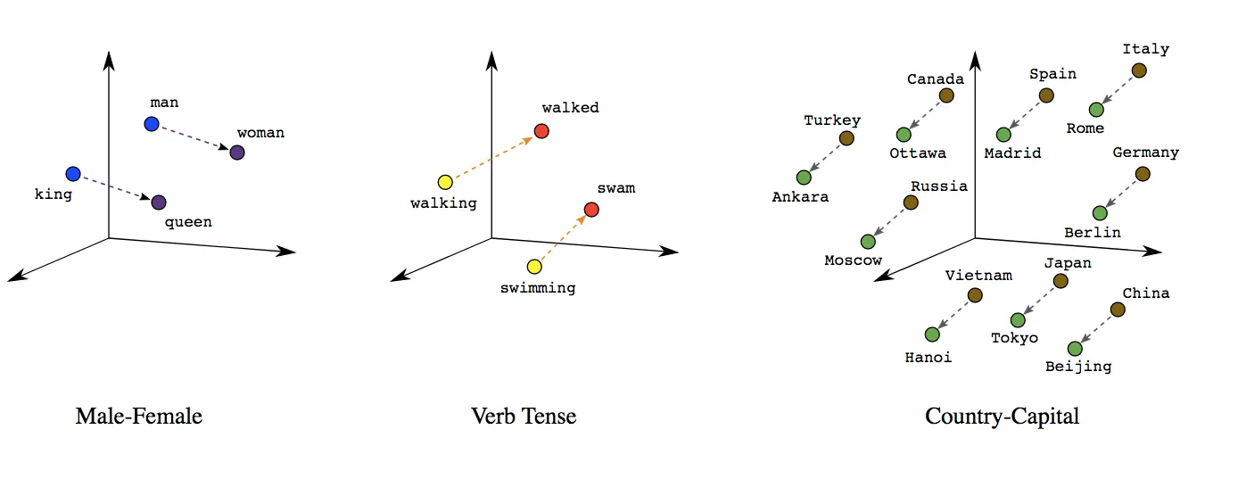
The famous example from Word2Vec:
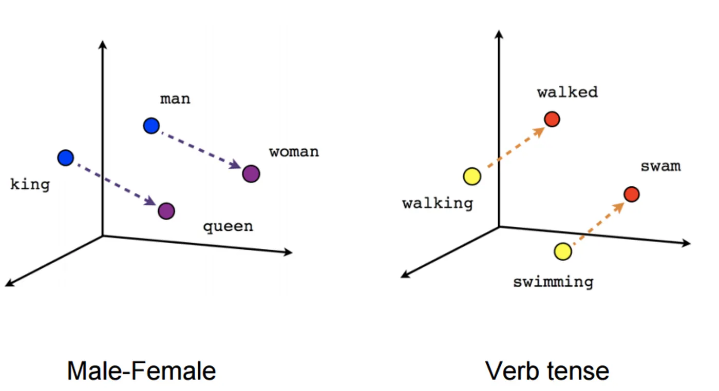
king - man + woman ≈ queen

E["king"] - E["man"] + E["woman"] ≈ E["queen"]

Numerically:
[0.52, 0.93, -0.12, 0.45]     # king
- [0.30, 0.85, -0.20, 0.15]   # man
+ [0.25, 0.70, -0.05, 0.35]   # woman
= [0.47, 0.78, -0.07, 0.65]   # ≈ queen
This works because:
king - mancaptures the concept of "royalty"- Adding
womanplaces us at the female version of royalty
Cosine Similarity measures how similar two embeddings are:
Example:
cat = [0.5, 0.6, 0.7, 0.8]
dog = [0.52, 0.58, 0.72, 0.79]  # Similar to cat
car = [0.1, -0.5, 0.2, 0.9]     # Different from cat

cosine_sim(cat, dog) = 0.998  # Very similar!
cosine_sim(cat, car) = 0.543 # Less similarThe choice of embedding dimension affects the model's capacity:
| Model | Embedding Dim | Parameters (for 50K vocab) |
|---|---|---|
| Small | 64 | 3.2M |
| Educational (this repo) | 128 | 6.4M |
| GPT-2 Small | 768 | 38.4M |
| GPT-2 Large | 1280 | 64M |
| GPT-3 | 12,288 | 614M |
| Small Embedding Dim | Large Embedding Dim |
|---|---|
| Fewer parameters | More parameters |
| Faster training | Slower training |
| Less capacity | More capacity |
| May underfit | May overfit (on small data) |
From src/layers.py, here's the Embedding class:
class Embedding:
    """
    Token Embedding Layer.

    Maps discrete token IDs to dense vector representations.
    This is essentially a learnable lookup table.

    Attributes:
        vocabulary_size: Number of unique tokens
        embedding_dimension: Size of embedding vectors
        embedding_table: The learnable weight matrix (vocab_size, embed_dim)
    """

    def __init__(self, vocabulary_size: int, embedding_dimension: int):
        """
        Initialize embedding layer with Xavier initialization.

        Args:
            vocabulary_size: Number of tokens in vocabulary
            embedding_dimension: Dimension of embedding vectors
        """
        self.vocabulary_size = vocabulary_size
        self.embedding_dimension = embedding_dimension

        # Initialize embedding table with Xavier/Glorot initialization
        # This helps maintain variance across layers
        weight_std = np.sqrt(2.0 / (vocabulary_size + embedding_dimension))
        self.embedding_table = np.random.randn(
            vocabulary_size, embedding_dimension
        ) * weight_std

        # Cache for backward pass
        self._input_cache = None
        self.embedding_gradient = None

    def forward(self, token_ids: np.ndarray) -> np.ndarray:
        """
        Look up embeddings for input token IDs.

        Args:
            token_ids: Integer array of shape (batch_size, sequence_length)

        Returns:
            Embeddings of shape (batch_size, sequence_length, embedding_dim)

        The operation is simply: output[b, t, :] = embedding_table[token_ids[b, t], :]
        """
        self._input_cache = token_ids

        # Simple indexing performs the lookup
        return self.embedding_table[token_ids]

    def backward(self, upstream_gradient: np.ndarray) -> None:
        """
        Compute gradient for embedding table.

        The gradient for each embedding vector is the sum of upstream
        gradients for all positions where that token appears.

        Args:
            upstream_gradient: Shape (batch_size, seq_len, embedding_dim)
        """
        token_ids = self._input_cache

        # Initialize gradient to zeros
        self.embedding_gradient = np.zeros_like(self.embedding_table)

        # Accumulate gradients for each token
        # If token i appears multiple times, its gradients are summed
        batch_size, seq_len = token_ids.shape
        for b in range(batch_size):
            for t in range(seq_len):
                token_id = token_ids[b, t]
                self.embedding_gradient[token_id] += upstream_gradient[b, t]

    @property
    def weight(self) -> np.ndarray:
        """Return embedding table (for compatibility)."""
return self.embedding_tableimport numpy as np
from src.layers import Embedding
# Create embedding layer
vocab_size = 2000
embed_dim = 128
embedding = Embedding(vocab_size, embed_dim)
# Input: batch of token IDs
token_ids = np.array([
[42, 156, 89], # "The cat sat"
[42, 201, 89] # "The dog sat"
]) # Shape: (2, 3)
# Forward pass: lookup embeddings
embeddings = embedding.forward(token_ids)
print(f"Output shape: {embeddings.shape}") # (2, 3, 128)
# Each position now has a 128-dimensional vector
print(f"Embedding for token 42 (position 0,0): {embeddings[0, 0, :5]}...")
print(f"Embedding for token 42 (position 1,0): {embeddings[1, 0, :5]}...")
# These are identical because it's the same token! Embedding Dimension (128)
←─────────────────────────→
┌─────────────────────────────────┐
0 │▓▓▓░░▓░░▓▓░░░▓▓░▓░░░▓░▓░░▓░▓░│ <PAD>
1 │░▓▓░░░▓▓░░▓░▓░░▓▓░▓▓░░░▓░▓▓░░│ <UNK>
2 │▓░▓░▓▓░░░▓░▓▓░░░▓░▓▓░░▓░░▓░▓░│ <BOS>
V : │ ... │
o : │ ... │
c 156 │▓▓░░▓░▓▓░░▓░░░▓▓▓░░▓░░▓▓░░▓░▓│ "cat"
a 157 │▓▓░░▓░▓▓░▓▓░░░▓▓▓░░▓░░▓░░░▓░▓│ "dog" (similar to cat!)
b : │ ... │
: │ ... │
(2000) 1999│░▓░▓░░▓░▓▓▓░░▓░░▓▓░░▓░▓░░▓▓░░│ last token
└─────────────────────────────────┘
▓ = positive value, ░ = negative value
                    2D Projection of Embedding Space

                              Animals
                              ╭─────╮
                         "cat" ●   ● "dog"
                      "kitten" ●     ● "puppy"
                              ╰─────╯

        Royalty                               Actions
        ╭─────╮                               ╭─────╮
   "king" ●   ● "queen"              "ran" ●    ● "walked"
  "prince" ●   ● "princess"          "ate" ●    ● "drank"
        ╰─────╯                               ╰─────╯

                              Places
                              ╭─────╮
                       "city" ●   ● "town"
                     "country" ●   ● "nation"
                              ╰─────╯
Input: "The cat sat"

Token IDs:      [42]         [156]        [89]
                 │            │            │
                 ▼            ▼            ▼
            ┌────────────────────────────────────┐
            │        Embedding Table             │
            │    (vocab_size × embed_dim)        │
            └────────────────────────────────────┘
                 │            │            │
                 ▼            ▼            ▼
Embeddings: [0.12,...]   [0.45,...]   [0.33,...]
            (128-dim)    (128-dim)    (128-dim)
                 │            │            │
                 └────────────┼────────────┘
                              │
                              ▼
              Stack into (1, 3, 128) tensor
                              │
                              ▼
              + Positional Encoding
                              │
                              ▼
              To Transformer Layers...
Embeddings are learned during training through backpropagation:
# Token "cat" (ID 156) appears in the input
embedding = E[156]  # Look up the embedding

# This embedding flows through the network
output = model(embedding)
loss = compute_loss(output, target)# Gradient flows back to the embedding
d_embedding = backprop(loss)
# Update only the embedding for token 156
E[156] -= learning_rate * d_embeddingIf a token appears multiple times:
Input: "the cat and the dog"
Token IDs: [42, 156, 89, 42, 201]
           "the"       "the"

The gradient for token 42 ("the") is the SUM of gradients
from both position 0 and position 3.
Some models "tie" the embedding weights with the output projection:
Embedding (input):  token_id → embedding_vector  (E)
Output projection:  hidden_state → logits over vocab (W)

With weight tying: W = E^T

Benefits:
- Fewer parameters (significant for large vocabs)
- Encourages semantic consistency
Run the layers demo to see embeddings in action:
python -m src.layersOr experiment in Python:
from src.layers import Embedding
import numpy as np

# Create embedding layer
embed = Embedding(vocabulary_size=1000, embedding_dimension=64)

# Test lookup
tokens = np.array([[1, 2, 3], [4, 5, 6]])
embeddings = embed.forward(tokens)
print(f"Input shape: {tokens.shape}")
print(f"Output shape: {embeddings.shape}")

# Check that same tokens get same embeddings
tokens_repeated = np.array([[1, 1, 1]])
emb_repeated = embed.forward(tokens_repeated)
print(f"Same embeddings? {np.allclose(emb_repeated[0,0], emb_repeated[0,1])}")

# Measure similarity between two embeddings
def cosine_similarity(a, b):
    return np.dot(a, b) / (np.linalg.norm(a) * np.linalg.norm(b))

emb1 = embed.embedding_table[100]
emb2 = embed.embedding_table[101]
print(f"Cosine similarity (before training): {cosine_similarity(emb1, emb2):.3f}")-
Word2Vec Paper: Mikolov, T., et al. (2013). Efficient Estimation of Word Representations in Vector Space
-
GloVe: Pennington, J., et al. (2014). GloVe: Global Vectors for Word Representation
-
StatQuest Word Embeddings Video: Word Embedding and Word2Vec, Clearly Explained!!!
-
IBM Explanation: What Are Word Embeddings?
-
Weaviate Blog: Vector Embeddings Explained
-
This Repository: See src/layers.py for the
Embeddingclass implementation.
Next Step: Embeddings don't carry position information - "cat sat" and "sat cat" would have identical embeddings (just in different order). Continue to 03 - PositionalEncoding.md to learn how we add position information.