The attention mechanism is what makes transformers powerful. It allows each token to "look at" all other tokens and decide which ones are relevant for understanding its context. This is the key innovation that enables modern language models.
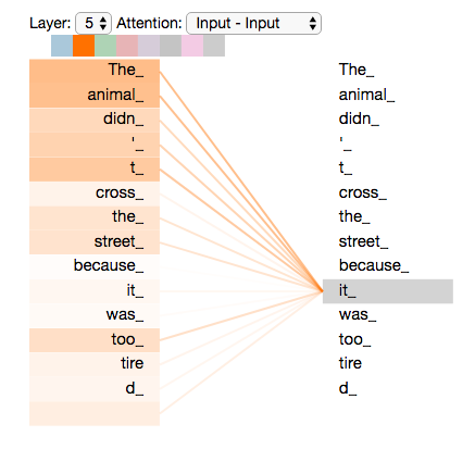
- What Is Attention?
- Query, Key, Value: The Core Intuition
- Scaled Dot-Product Attention
- Step-by-Step Numeric Example
- Causal Masking
- Multi-Head Attention
- Code Implementation
- Visualization
- References
Attention is a mechanism that allows the model to focus on relevant parts of the input when producing each part of the output.
When you read the sentence "The cat that ran across the street was black", your brain automatically connects "cat" with "black" despite the words in between. This is attention - focusing on the relevant information.
Without attention:
- Each position only sees local context (like in CNNs) or
- Information must flow sequentially (like in RNNs)
With attention:
- Every position can directly access every other position
- Long-range dependencies are captured in one step
- Parallel computation is possible
The attention mechanism uses three projections of the input: Query (Q), Key (K), and Value (V).
Think of attention like searching a database:
| Concept | Database Analogy | In Attention |
|---|---|---|
| Query (Q) | Search term: "What am I looking for?" | Current token asking for context |
| Key (K) | Index/tag: "What does each record contain?" | Each token's identifier |
| Value (V) | Content: "The actual information" | Each token's information to retrieve |
- Each token creates a Query: "What information do I need?"
- Each token also creates a Key and Value
- We compare the Query against all Keys to get attention scores
- High-scoring Keys have their Values contribute more to the output
Sentence: "The cat sat on the mat"

When processing "sat":
  Query for "sat" asks: "Who performed the action?"

  Token    | Key (what it is)     | Attention Score | Value (its info)
  ---------|----------------------|-----------------|------------------
  "The"    | article              | 0.05 (low)      | [0.1, 0.2, ...]
  "cat"    | noun, subject        | 0.60 (HIGH!)    | [0.5, 0.8, ...]
  "sat"    | verb, current        | 0.20 (medium)   | [0.3, 0.4, ...]
  "on"     | preposition          | 0.10 (low)      | [0.2, 0.1, ...]
  "the"    | article              | 0.03 (low)      | [0.1, 0.2, ...]
  "mat"    | noun, object         | 0.02 (low)      | [0.4, 0.3, ...]
                                    ↓
  Output = weighted sum of Values = mostly "cat"'s information
Where:
-
$Q$ = Query matrix (what each position is looking for) -
$K$ = Key matrix (what each position contains) -
$V$ = Value matrix (what information each position provides) -
$d_k$ = dimension of keys (for scaling)
Step 1: QK^T           → Compute similarity between queries and keys
Step 2: / sqrt(d_k)    → Scale down to prevent extreme values
Step 3: softmax        → Convert to probability distribution
Step 4: × V            → Weighted combination of values
Without scaling, dot products grow with dimension:
d_k = 64:  dot product variance ≈ 64
d_k = 512: dot product variance ≈ 512
Large values push softmax into regions with tiny gradients:
softmax([100, 1, 1, 1]) ≈ [1.0, 0.0, 0.0, 0.0]  # Gradient ≈ 0!
softmax([2, 0.5, 0.5, 0.5]) ≈ [0.5, 0.17, 0.17, 0.17]  # Better gradients
Scaling by
Let's compute attention for a tiny example:
Sequence: ["cat", "sat", "mat"]  (3 tokens)
Embedding dimension: 4
Query/Key dimension (d_k): 4
Value dimension (d_v): 4
X = [
    [1.0, 0.5, 0.2, 0.8],  # "cat"
    [0.3, 0.9, 0.1, 0.4],  # "sat"
    [0.6, 0.2, 0.7, 0.3],  # "mat"
]
# Shape: (3, 4)# Weight matrices (simplified - normally learned)
W_Q = [[1, 0, 0, 0],
[0, 1, 0, 0],
[0, 0, 1, 0],
[0, 0, 0, 1]] # Identity for simplicity
W_K = W_V = W_Q # Same for this example
# Compute projections: Q = X @ W_Q^T
Q = X @ W_Q.T # Same as X in this case
K = X @ W_K.T
V = X @ W_V.T
# Q, K, V all equal X in this simplified example:
Q = K = V = [
[1.0, 0.5, 0.2, 0.8], # "cat"
[0.3, 0.9, 0.1, 0.4], # "sat"
[0.6, 0.2, 0.7, 0.3], # "mat"
]# scores[i][j] = Q[i] · K[j] (dot product)
scores = Q @ K.T
# Computing each element:
# scores[0][0] = Q[0] · K[0] = 1.0*1.0 + 0.5*0.5 + 0.2*0.2 + 0.8*0.8 = 1.93
# scores[0][1] = Q[0] · K[1] = 1.0*0.3 + 0.5*0.9 + 0.2*0.1 + 0.8*0.4 = 1.09
# scores[0][2] = Q[0] · K[2] = 1.0*0.6 + 0.5*0.2 + 0.2*0.7 + 0.8*0.3 = 1.08
# ... and so on
scores = [
[1.93, 1.09, 1.08], # "cat" attending to all
[1.09, 1.07, 0.65], # "sat" attending to all
[1.08, 0.65, 0.98], # "mat" attending to all
]d_k = 4
sqrt_d_k = 2.0
scaled_scores = scores / sqrt_d_k
scaled_scores = [
[0.965, 0.545, 0.540],
[0.545, 0.535, 0.325],
[0.540, 0.325, 0.490],
]# softmax converts each row to probability distribution
# softmax(x_i) = exp(x_i) / sum(exp(x_j))
attention_weights = softmax(scaled_scores, axis=-1)
# For row 0: [0.965, 0.545, 0.540]
# exp([0.965, 0.545, 0.540]) = [2.625, 1.725, 1.716]
# sum = 6.066
# [2.625/6.066, 1.725/6.066, 1.716/6.066] = [0.433, 0.284, 0.283]
attention_weights = [
[0.433, 0.284, 0.283], # "cat": 43% self, 28% "sat", 28% "mat"
[0.384, 0.377, 0.239], # "sat": 38% "cat", 38% self, 24% "mat"
[0.389, 0.269, 0.342], # "mat": 39% "cat", 27% "sat", 34% self
]# output[i] = sum(attention_weights[i][j] * V[j])
# For "cat" (position 0):
output[0] = 0.433 * V[0] + 0.284 * V[1] + 0.283 * V[2]
= 0.433 * [1.0, 0.5, 0.2, 0.8]
+ 0.284 * [0.3, 0.9, 0.1, 0.4]
+ 0.283 * [0.6, 0.2, 0.7, 0.3]
= [0.433, 0.217, 0.087, 0.347]
+ [0.085, 0.256, 0.028, 0.114]
+ [0.170, 0.057, 0.198, 0.085]
= [0.688, 0.530, 0.313, 0.546]
# Full output matrix:
output = [
[0.688, 0.530, 0.313, 0.546], # "cat" with context
[0.644, 0.529, 0.279, 0.538], # "sat" with context
[0.666, 0.477, 0.330, 0.543], # "mat" with context
]Each output row is now a context-aware representation that incorporates information from relevant tokens!
For autoregressive language models (like GPT), we can only look at past tokens, not future ones.
During training, we predict each token from previous tokens only:
"The cat sat" → predict each word from left context

Position 0: predict "The" from nothing (or <BOS>)
Position 1: predict "cat" from "The"
Position 2: predict "sat" from "The cat"
If position 2 could see "sat", it would be cheating!
# For sequence length 4:
causal_mask = [
    [True,  False, False, False],  # pos 0 sees only itself
    [True,  True,  False, False],  # pos 1 sees 0, 1
    [True,  True,  True,  False],  # pos 2 sees 0, 1, 2
    [True,  True,  True,  True],   # pos 3 sees 0, 1, 2, 3
]

# Applied to attention scores BEFORE softmax:
masked_scores = where(mask, scores, -infinity)

# Example:
# Original scores for position 2: [0.5, 0.8, 0.3, 0.9]
# After masking:                  [0.5, 0.8, 0.3, -inf]
# After softmax:                  [0.28, 0.41, 0.31, 0.00]
# ↑ can't see future! Keys (what we're looking at)
┌───────────────────────────────┐
│ pos0 pos1 pos2 pos3 │
┌─────┼───────────────────────────────┤
│pos0 │ ✓ ✗ ✗ ✗ │
Queries │pos1 │ ✓ ✓ ✗ ✗ │
(who's │pos2 │ ✓ ✓ ✓ ✗ │
looking)│pos3 │ ✓ ✓ ✓ ✓ │
└─────┴───────────────────────────────┘
✓ = can attend (visible)
✗ = masked out (set to -∞ before softmax)
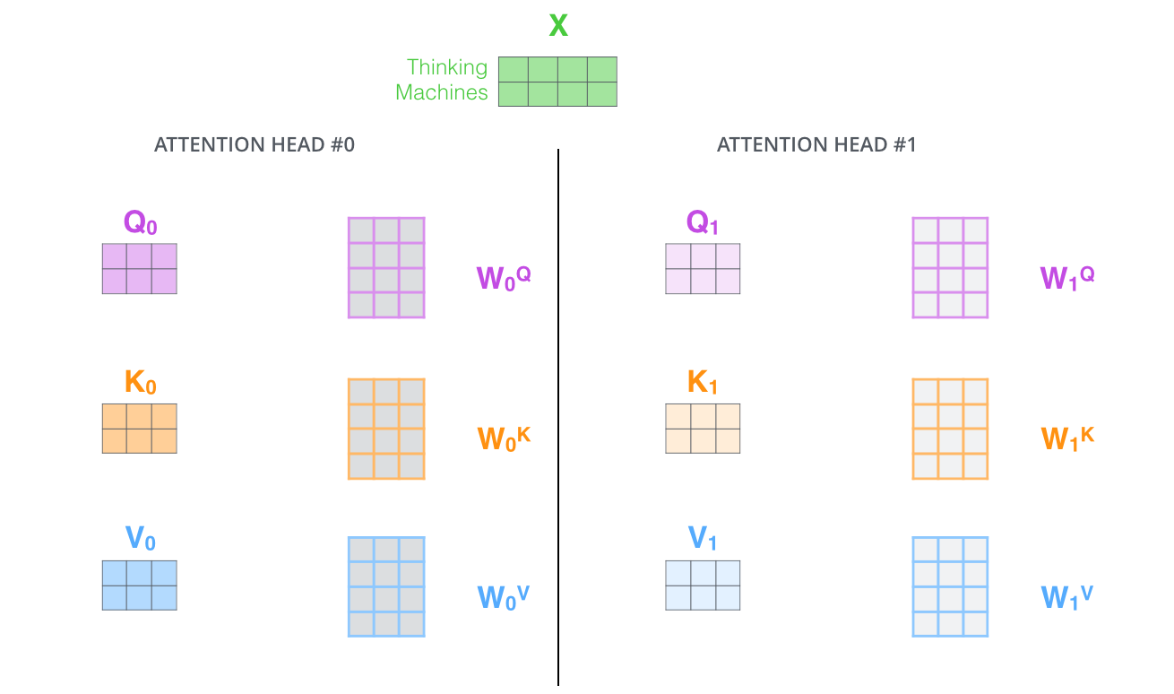
Instead of one attention function, we run multiple attention heads in parallel.
Different heads can learn different patterns:
- Head 1: Focus on grammatical relationships (subject-verb)
- Head 2: Focus on nearby context
- Head 3: Focus on semantic similarity
- Head 4: Focus on specific phrases or patterns
Input X (embed_dim = 128)
         │
         ├─────────────────────────────────┐
         │                                 │
    Split into 4 heads                     │
    (each head: dim = 32)                  │
         │                                 │
   ┌─────┴─────┬─────┬─────┐               │
   ▼           ▼     ▼     ▼               │
Head 1     Head 2  Head 3  Head 4          │
(32-d)     (32-d)  (32-d)  (32-d)          │
   │           │     │     │               │
   └─────┬─────┴─────┴─────┘               │
         │                                 │
   Concatenate (128-d)                     │
         │                                 │
   Linear projection (128 → 128)           │
         │                                 │
         ▼                                 │
   Multi-Head Output ──────────────────────┘
Where each head is:
# Model dimensions
embed_dim = 128
num_heads = 4
head_dim = embed_dim // num_heads  # 32

# Input shape: (batch, seq_len, 128)

# Step 1: Project Q, K, V
Q = X @ W_Q  # (batch, seq_len, 128)
K = X @ W_K
V = X @ W_V

# Step 2: Split into heads
# Reshape: (batch, seq_len, 128) → (batch, seq_len, 4, 32)
# Transpose: → (batch, 4, seq_len, 32)
Q = Q.reshape(batch, seq_len, 4, 32).transpose(0, 2, 1, 3)
K = K.reshape(batch, seq_len, 4, 32).transpose(0, 2, 1, 3)
V = V.reshape(batch, seq_len, 4, 32).transpose(0, 2, 1, 3)

# Step 3: Apply attention per head
# Each head computes attention independently with 32-d vectors
head_outputs = []
for h in range(4):
    head_out = scaled_dot_product_attention(Q[:, h], K[:, h], V[:, h])
    head_outputs.append(head_out)  # Each: (batch, seq_len, 32)

# Step 4: Concatenate heads
concat = concatenate(head_outputs, dim=-1)  # (batch, seq_len, 128)

# Step 5: Final projection
output = concat @ W_O # (batch, seq_len, 128)From src/attention.py:
def scaled_dot_product_attention(
    query: np.ndarray,
    key: np.ndarray,
    value: np.ndarray,
    mask: Optional[np.ndarray] = None,
) -> Tuple[np.ndarray, np.ndarray]:
    """
    Compute Scaled Dot-Product Attention.

    Attention(Q, K, V) = softmax(Q @ K^T / sqrt(d_k)) @ V

    Args:
        query: Shape (batch_size, seq_len_q, d_k)
        key: Shape (batch_size, seq_len_k, d_k)
        value: Shape (batch_size, seq_len_k, d_v)
        mask: Optional boolean mask

    Returns:
        output: Shape (batch_size, seq_len_q, d_v)
        attention_weights: Shape (batch_size, seq_len_q, seq_len_k)
    """
    d_k = query.shape[-1]

    # Step 1: QK^T
    attention_scores = np.matmul(query, key.transpose(0, 2, 1))

    # Step 2: Scale
    scaled_attention_scores = attention_scores / np.sqrt(d_k)

    # Step 3: Apply mask
    if mask is not None:
        if mask.ndim == 2:
            mask = mask[np.newaxis, :, :]
        scaled_attention_scores = np.where(mask, scaled_attention_scores, -1e9)

    # Step 4: Softmax
    attention_weights = softmax(scaled_attention_scores, axis=-1)

    # Step 5: Weighted sum of values
    attention_output = np.matmul(attention_weights, value)

return attention_output, attention_weightsclass MultiHeadAttention:
"""
Multi-Head Attention Layer.
Performs attention multiple times in parallel with different
learned projections, then combines the results.
"""
def __init__(self, embedding_dimension: int, num_heads: int):
self.embedding_dimension = embedding_dimension
self.num_heads = num_heads
self.head_dimension = embedding_dimension // num_heads
# Projection layers
self.query_projection = Linear(embedding_dimension, embedding_dimension)
self.key_projection = Linear(embedding_dimension, embedding_dimension)
self.value_projection = Linear(embedding_dimension, embedding_dimension)
self.output_projection = Linear(embedding_dimension, embedding_dimension)
def forward(self, query, key, value, mask=None):
batch_size = query.shape[0]
seq_len_q = query.shape[1]
seq_len_k = key.shape[1]
# Project Q, K, V
Q = self.query_projection.forward(query)
K = self.key_projection.forward(key)
V = self.value_projection.forward(value)
# Reshape for multi-head: (batch, seq, embed) → (batch, heads, seq, head_dim)
Q = Q.reshape(batch_size, seq_len_q, self.num_heads, self.head_dimension)
Q = Q.transpose(0, 2, 1, 3)
K = K.reshape(batch_size, seq_len_k, self.num_heads, self.head_dimension)
K = K.transpose(0, 2, 1, 3)
V = V.reshape(batch_size, seq_len_k, self.num_heads, self.head_dimension)
V = V.transpose(0, 2, 1, 3)
# Attention per head
attn_output, attn_weights = scaled_dot_product_attention(Q, K, V, mask)
# Concatenate heads
attn_output = attn_output.transpose(0, 2, 1, 3)
attn_output = attn_output.reshape(batch_size, seq_len_q, self.embedding_dimension)
# Final projection
output = self.output_projection.forward(attn_output)
return outputAttending to: "The cat sat on the mat"
│ The cat sat on the mat │
─────┼───────────────────────────────┤
The │ ▓▓▓ ░░ ░░ ░░ ░░ ░░ │ mostly self
cat │ ░░ ▓▓▓ ░░ ░░ ░░ ▓░ │ self + "mat"
sat │ ░░ ▓▓▓ ▓▓ ░░ ░░ ░░ │ "cat" is subject
on │ ░░ ░░ ▓░ ▓░ ░░ ░░ │ "sat" context
the │ ░░ ░░ ░░ ░░ ▓▓ ░░ │ mostly self
mat │ ░░ ▓░ ▓░ ▓░ ░░ ▓▓ │ contextual
─────┴───────────────────────────────┘
▓▓▓ = high attention (>0.3)
░░ = low attention (<0.1)
Head 1 (Grammar):           Head 2 (Recent):          Head 3 (Semantic):
┌────────────────┐          ┌────────────────┐        ┌────────────────┐
│▓▓▓░░░░░░░░░░░░│          │▓▓▓▓▓▓░░░░░░░░│        │▓░▓▓░░░░░▓░░░░│
│░░░▓▓▓░░░░░░░░░│          │░▓▓▓▓▓▓░░░░░░░│        │▓░░▓░░░░░░▓░░░│
│░▓░░░▓▓░░░░░░░░│ ←verb→   │░░▓▓▓▓▓▓░░░░░░│        │░░░░▓░░░░░░▓░░│
│░░░░▓░░▓░░░░░░░│  subject │░░░▓▓▓▓▓▓░░░░░│        │░░░░░░░░░░░░▓░│
│░░░░░░░░▓▓▓░░░░│          │░░░░▓▓▓▓▓▓░░░░│        │░░▓░░░░░░░░░▓▓│
└────────────────┘          └────────────────┘        └────────────────┘
   Subject-verb              Local context           Semantic similarity
Input: "The cat sat"
       ┌───┐  ┌───┐  ┌───┐
       │The│  │cat│  │sat│
       └─┬─┘  └─┬─┘  └─┬─┘
         │      │      │
    ┌────┴──────┴──────┴────┐
    │   Linear Projections   │
    │   Q = X·W_Q            │
    │   K = X·W_K            │
    │   V = X·W_V            │
    └────┬──────┬──────┬────┘
         │      │      │
         ▼      ▼      ▼
       ┌─────────────────────┐
       │ Q·K^T / √d_k        │  ← Compute similarities
       │ ┌─────────────────┐ │
       │ │ .8  .3  .2     │ │  Each row shows how much
       │ │ .2  .7  .3     │ │  each position attends
       │ │ .1  .6  .5     │ │  to each other position
       │ └─────────────────┘ │
       └──────────┬──────────┘
                  │
                  ▼
       ┌─────────────────────┐
       │ softmax(scores)     │  ← Normalize to probabilities
       │ ┌─────────────────┐ │
       │ │.50 .30 .20     │ │  Each row sums to 1.0
       │ │.20 .50 .30     │ │
       │ │.15 .45 .40     │ │
       │ └─────────────────┘ │
       └──────────┬──────────┘
                  │
                  ▼
       ┌─────────────────────┐
       │ weights × V          │  ← Weighted combination
       └──────────┬──────────┘
                  │
                  ▼
       ┌───┐  ┌───┐  ┌───┐
       │The│  │cat│  │sat│     Context-enriched
       │ + │  │ + │  │ + │     representations
       │ctx│  │ctx│  │ctx│
       └───┘  └───┘  └───┘
Run the attention demo:
python -m src.attentionOr experiment in Python:
from src.attention import scaled_dot_product_attention, create_causal_mask
import numpy as np

# Create sample Q, K, V
seq_len, d_k = 4, 8
batch_size = 1

np.random.seed(42)
Q = np.random.randn(batch_size, seq_len, d_k)
K = np.random.randn(batch_size, seq_len, d_k)
V = np.random.randn(batch_size, seq_len, d_k)

# Without mask (bidirectional)
output1, weights1 = scaled_dot_product_attention(Q, K, V)
print("Attention weights (no mask):")
print(weights1[0].round(2))

# With causal mask (autoregressive)
mask = create_causal_mask(seq_len)
output2, weights2 = scaled_dot_product_attention(Q, K, V, mask)
print("\nAttention weights (causal mask):")
print(weights2[0].round(2))

# Notice: with causal mask, lower triangle is populated
# upper triangle is zero (can't attend to future)-
Original Transformer Paper: Vaswani, A., et al. (2017). Attention Is All You Need
-
The Illustrated Transformer: Jay Alammar's Visual Guide
-
Dive into Deep Learning - Attention: d2l.ai Queries, Keys, and Values
-
Transformer Attention Guide: billparker.ai Q, K, V Matrices
-
3Blue1Brown Attention Video: Visualizing Attention
-
This Repository: See src/attention.py for complete implementation.
Next Step: Attention lets tokens communicate with each other. But we also need to process each token individually to add non-linearity. Continue to 05 - FeedForwardNetwork.md to learn about the FFN component.