After attention allows tokens to communicate, the Feed-Forward Network (FFN) processes each position independently. This is where the model applies non-linear transformations and stores much of its "knowledge."
- Purpose of the FFN
- Architecture
- The GELU Activation
- Step-by-Step Numeric Example
- Why Expand Then Contract?
- Code Implementation
- Visualization
- References
The Feed-Forward Network serves several crucial purposes:
Attention is essentially a weighted sum (linear operation). Without non-linearity, stacking layers wouldn't add expressiveness. The FFN adds the non-linear activation needed for complex function approximation.
While attention mixes information across positions, FFN processes each position independently. This allows position-specific transformations.
Attention: tokens talk to each other        FFN: each token thinks alone

    A ←→ B ←→ C ←→ D                          A → A'
         ↕                                     B → B'
    B ←→ C ←→ D                                C → C'
                                               D → D'
Research suggests that much of the "knowledge" in transformers is stored in FFN weights. The large hidden dimension provides capacity to memorize patterns and facts.
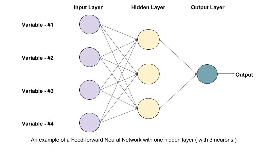
The FFN is a simple two-layer network:
Or in more detail:
Input:           x        shape: (batch, seq_len, d_model)     e.g., 128
                 ↓
Linear 1:   W_1 @ x + b_1  shape: (batch, seq_len, d_ff)       e.g., 512
                 ↓
GELU:       gelu(hidden)   shape: (batch, seq_len, d_ff)       e.g., 512
                 ↓
Linear 2:   W_2 @ h + b_2  shape: (batch, seq_len, d_model)    e.g., 128
                 ↓
Output:          y        shape: (batch, seq_len, d_model)     e.g., 128
The typical ratio is
GELU provides a smooth non-linearity compared to ReLU's sharp cutoff, allowing small negative values to pass through.
GELU (Gaussian Error Linear Unit) is the activation function used in GPT-2, GPT-3, BERT, and most modern transformers.
Where
Since computing the exact CDF is expensive, we use a tanh approximation:
                  GELU                              ReLU
        ▲                                   ▲
      3 │            ╱                    3 │            /
        │          ╱                        │          /
      2 │        ╱                        2 │        /
        │      ╱                            │      /
      1 │    ╱                            1 │    /
        │  ╱                                │  /
      0 │──────╮                          0 │────────────
        │      ╲                            │
     -1 │        ╲                       -1 │
        └──────────────────►              └──────────────────►
         -3  -2  -1   0   1   2   3         -3  -2  -1   0   1   2   3

    GELU: Smooth, allows small               ReLU: Sharp cutoff at 0
          negative values through                  Zero gradient for x<0
| Property | GELU | ReLU |
|---|---|---|
| Negative inputs | Small values pass through | Completely blocked (0) |
| Smoothness | Smooth everywhere | Sharp corner at 0 |
| Gradient for x < 0 | Non-zero | Zero (dead neurons) |
| Probabilistic interpretation | Input × probability of being positive | None |
| Input x | GELU(x) | ReLU(x) |
|---|---|---|
| -2.0 | -0.045 | 0.0 |
| -1.0 | -0.159 | 0.0 |
| -0.5 | -0.154 | 0.0 |
| 0.0 | 0.0 | 0.0 |
| 0.5 | 0.346 | 0.5 |
| 1.0 | 0.841 | 1.0 |
| 2.0 | 1.955 | 2.0 |
Let's trace through an FFN with small dimensions:
Input dimension (d_model):  4
Hidden dimension (d_ff):    8
Batch size:                 1
Sequence length:            2
# Linear 1: d_model (4) → d_ff (8)
W_1 = [
    [0.1, 0.2, 0.3, 0.4],   # 8 rows
    [0.2, 0.1, 0.4, 0.3],
    [0.3, 0.4, 0.1, 0.2],
    [0.4, 0.3, 0.2, 0.1],
    [0.1, 0.3, 0.2, 0.4],
    [0.2, 0.4, 0.1, 0.3],
    [0.3, 0.1, 0.4, 0.2],
    [0.4, 0.2, 0.3, 0.1],
]  # Shape: (8, 4)
b_1 = [0, 0, 0, 0, 0, 0, 0, 0]  # Shape: (8,)

# Linear 2: d_ff (8) → d_model (4)
W_2 = [
    [0.1, 0.2, 0.1, 0.2, 0.1, 0.2, 0.1, 0.2],   # 4 rows
    [0.2, 0.1, 0.2, 0.1, 0.2, 0.1, 0.2, 0.1],
    [0.1, 0.1, 0.2, 0.2, 0.1, 0.1, 0.2, 0.2],
    [0.2, 0.2, 0.1, 0.1, 0.2, 0.2, 0.1, 0.1],
]  # Shape: (4, 8)
b_2 = [0, 0, 0, 0] # Shape: (4,)x = [
[1.0, 0.5, -0.3, 0.8], # Position 0
[0.2, -0.4, 0.6, 0.1], # Position 1
] # Shape: (2, 4)For position 0: hidden[0] = W_1 @ x[0] + b_1
# x[0] = [1.0, 0.5, -0.3, 0.8]

hidden[0][0] = 0.1*1.0 + 0.2*0.5 + 0.3*(-0.3) + 0.4*0.8 = 0.43
hidden[0][1] = 0.2*1.0 + 0.1*0.5 + 0.4*(-0.3) + 0.3*0.8 = 0.37
hidden[0][2] = 0.3*1.0 + 0.4*0.5 + 0.1*(-0.3) + 0.2*0.8 = 0.63
hidden[0][3] = 0.4*1.0 + 0.3*0.5 + 0.2*(-0.3) + 0.1*0.8 = 0.57
hidden[0][4] = 0.1*1.0 + 0.3*0.5 + 0.2*(-0.3) + 0.4*0.8 = 0.51
hidden[0][5] = 0.2*1.0 + 0.4*0.5 + 0.1*(-0.3) + 0.3*0.8 = 0.61
hidden[0][6] = 0.3*1.0 + 0.1*0.5 + 0.4*(-0.3) + 0.2*0.8 = 0.39
hidden[0][7] = 0.4*1.0 + 0.2*0.5 + 0.3*(-0.3) + 0.1*0.8 = 0.49

hidden[0] = [0.43, 0.37, 0.63, 0.57, 0.51, 0.61, 0.39, 0.49]
Similarly for position 1:
hidden[1] = [0.17, 0.21, 0.23, 0.19, 0.20, 0.22, 0.29, 0.23]Full hidden: Shape (2, 8)
For each value
# For hidden[0] = [0.43, 0.37, 0.63, 0.57, 0.51, 0.61, 0.39, 0.49]

gelu(0.43) = 0.5 * 0.43 * (1 + tanh(0.7979 * (0.43 + 0.044715 * 0.43³)))
           = 0.5 * 0.43 * (1 + tanh(0.3465))
           = 0.5 * 0.43 * (1 + 0.333)
           = 0.287

activated[0] = [0.287, 0.241, 0.452, 0.400, 0.344, 0.432, 0.257, 0.328]
activated[1] = [0.098, 0.126, 0.140, 0.113, 0.121, 0.134, 0.182, 0.139]For position 0: output[0] = W_2 @ activated[0] + b_2
# activated[0] = [0.287, 0.241, 0.452, 0.400, 0.344, 0.432, 0.257, 0.328]

output[0][0] = 0.1*0.287 + 0.2*0.241 + 0.1*0.452 + 0.2*0.400 + ...
             = 0.498  (weighted sum of all 8 values)
output[0][1] = 0.492
output[0][2] = 0.489
output[0][3] = 0.501

output[0] = [0.498, 0.492, 0.489, 0.501]
output[1] = [0.187, 0.184, 0.182, 0.189]Input (d_model=4): [1.0, 0.5, -0.3, 0.8]
↓
Expand to d_ff=8: [0.43, 0.37, 0.63, 0.57, 0.51, 0.61, 0.39, 0.49]
↓
Apply GELU: [0.29, 0.24, 0.45, 0.40, 0.34, 0.43, 0.26, 0.33]
↓
Compress to d_model=4:[0.50, 0.49, 0.49, 0.50]
d_model = 128          d_ff = 512          d_model = 128
┌─────────┐         ┌────────────┐         ┌─────────┐
│         │         │            │         │         │
│   128   │   →     │    512     │    →    │   128   │
│         │         │            │         │         │
└─────────┘         └────────────┘         └─────────┘
  Compact            Expanded               Compact
  representation     processing space       representation
- More capacity: 512 neurons can learn more patterns than 128
- Sparse activation: After GELU, some neurons effectively "turn off"
- Feature disentanglement: Expand to process, then compress to essential features
The contraction step forces the network to:
- Compress information back to compact form
- Keep only the most important transformed features
- Discard noise introduced by expansion
Linear 1: d_model × d_ff + d_ff   = 128 × 512 + 512   = 66,048
Linear 2: d_ff × d_model + d_model = 512 × 128 + 128   = 65,664
Total:                                                 = 131,712

Compare to attention (Q, K, V, O projections):
4 × (128 × 128 + 128) = 66,048

FFN has ~2× the parameters of attention!
From src/transformer.py:
class FeedForwardNetwork:
    """
    Position-wise Feed-Forward Network.

    FFN(x) = Linear_2(GELU(Linear_1(x)))

    This is applied independently to each position in the sequence.
    The hidden dimension is typically 4x the model dimension.
    """

    def __init__(self, embedding_dimension: int, hidden_dimension: int = None):
        self.embedding_dimension = embedding_dimension
        self.hidden_dimension = hidden_dimension or (4 * embedding_dimension)

        # First linear: expand from d_model to d_ff
        self.linear_1 = Linear(
            input_features=embedding_dimension,
            output_features=self.hidden_dimension
        )

        # Second linear: compress from d_ff back to d_model
        self.linear_2 = Linear(
            input_features=self.hidden_dimension,
            output_features=embedding_dimension
        )

        # Caches for backward pass
        self._input_cache = None
        self._hidden_cache = None
        self._activated_cache = None

    def forward(self, input_tensor: np.ndarray) -> np.ndarray:
        """
        Forward pass through FFN.

        Args:
            input_tensor: Shape (batch, seq_len, embedding_dim)

        Returns:
            Output of same shape
        """
        self._input_cache = input_tensor

        # Step 1: Expand to hidden dimension
        hidden = self.linear_1.forward(input_tensor)
        self._hidden_cache = hidden

        # Step 2: Apply GELU activation
        activated = gelu(hidden)
        self._activated_cache = activated

        # Step 3: Compress back to embedding dimension
        output = self.linear_2.forward(activated)

        return output

    def backward(self, upstream_gradient: np.ndarray) -> np.ndarray:
        """
        Backward pass through FFN.
        """
        # Backward through linear_2
        d_activated = self.linear_2.backward(upstream_gradient)

        # Backward through GELU
        d_hidden = gelu_backward(d_activated, self._hidden_cache)

        # Backward through linear_1
        d_input = self.linear_1.backward(d_hidden)

return d_inputFrom src/activations.py:
def gelu(x: np.ndarray) -> np.ndarray:
    """
    Gaussian Error Linear Unit.

    GELU(x) ≈ 0.5 * x * (1 + tanh(sqrt(2/pi) * (x + 0.044715 * x^3)))

    This is the activation function used in GPT-2, GPT-3, and BERT.
    """
    sqrt_2_over_pi = np.sqrt(2.0 / np.pi)  # ≈ 0.7979
    cubic_coefficient = 0.044715

    # Compute inner expression
    cubic_term = cubic_coefficient * np.power(x, 3)
    inner_expression = sqrt_2_over_pi * (x + cubic_term)

    # Apply tanh and scale
    tanh_result = np.tanh(inner_expression)
    gelu_output = 0.5 * x * (1.0 + tanh_result)

    return gelu_output


def gelu_backward(upstream_gradient: np.ndarray, x: np.ndarray) -> np.ndarray:
    """
    Gradient of GELU.

    d(GELU)/dx = 0.5*(1 + tanh(z)) + 0.5*x*sech²(z)*dz/dx

    where z = sqrt(2/π)*(x + 0.044715*x³)
          dz/dx = sqrt(2/π)*(1 + 3*0.044715*x²)
    """
    sqrt_2_over_pi = np.sqrt(2.0 / np.pi)
    c = 0.044715

    # Forward values
    z = sqrt_2_over_pi * (x + c * x**3)
    tanh_z = np.tanh(z)

    # Derivative of z
    dz_dx = sqrt_2_over_pi * (1 + 3 * c * x**2)

    # sech²(z) = 1 - tanh²(z)
    sech2_z = 1 - tanh_z**2

    # Full gradient
    gelu_grad = 0.5 * (1 + tanh_z) + 0.5 * x * sech2_z * dz_dx

return upstream_gradient * gelu_grad Embedding Dimension (128)
┌───────────────────────────┐
Input │░░░░░░░░░░░░░░░░░░░░░░░░░░░│
└────────────┬──────────────┘
│
Linear_1 (W₁)
(expand 128→512)
│
▼
Hidden Dimension (512)
┌────────────────────────────────────────────────────────────────────────┐
│▓▓▓▓▓▓▓▓▓▓▓▓▓▓▓▓▓▓▓▓▓▓▓▓▓▓▓▓▓▓▓▓▓▓▓▓▓▓▓▓▓▓▓▓▓▓▓▓▓▓▓▓▓▓▓▓▓▓▓▓▓▓▓▓▓▓▓▓│
└────────────────────────────────┬───────────────────────────────────────┘
│
GELU
│
▼
┌────────────────────────────────────────────────────┐
After GELU │▓▓▓▓░░▓▓▓▓▓░░░░▓▓▓░░▓▓▓░░░░▓▓░░░░▓▓▓▓▓░░░▓▓▓▓░░░│
└────────────────────────┬───────────────────────────┘
│ Some neurons near zero
Linear_2 (W₂) (sparse activation)
(compress 512→128)
│
▼
┌───────────────────────────┐
Output │░▓▓░▓░░▓▓░░▓░░▓▓░░▓▓░░░▓▓░│
└───────────────────────────┘
Embedding Dimension (128)
Input values across hidden dimension (512):

Before GELU:
─2.0│    ╭─╮       ╭───╮                  ╭─╮
─1.0│  ╭─╯ │   ╭───╯   ╰──╮           ╭───╯ │
 0.0│──╯   ╰───╯          ╰───────────╯     ╰──
+1.0│
+2.0│
    └────────────────────────────────────────────────
                   Hidden Dimension →

After GELU:
─2.0│
─1.0│
 0.0│──────────────────────────────────────────  Most negatives ≈ 0
+1.0│    ╭─╮       ╭───╮                  ╭─╮    Positives preserved
+2.0│  ╭─╯ │   ╭───╯   ╰──╮           ╭───╯ │
    └────────────────────────────────────────────────
                   Hidden Dimension →
Sequence: "The" "cat" "sat"
              │     │     │
              ▼     ▼     ▼
         ┌────────────────────┐
         │                    │ Each position
Input    │  [128] [128] [128] │ processed
         │                    │ independently
         └─────┬──────┬──────┬┘
               │      │      │
         ┌─────▼─┐┌───▼───┐┌─▼─────┐
         │ FFN   ││ FFN   ││ FFN   │  Same weights,
         │(same) ││(same) ││(same) │  different inputs
         └─────┬─┘└───┬───┘└─┬─────┘
               │      │      │
               ▼      ▼      ▼
         ┌────────────────────┐
Output   │  [128] [128] [128] │
         └────────────────────┘
Run the transformer demo to see FFN in action:
python -m src.transformerOr experiment in Python:
from src.transformer import FeedForwardNetwork
from src.activations import gelu
import numpy as np

# Create FFN
ffn = FeedForwardNetwork(embedding_dimension=128, hidden_dimension=512)

# Sample input
x = np.random.randn(1, 10, 128)  # batch=1, seq=10, dim=128

# Forward pass
output = ffn.forward(x)
print(f"Input shape: {x.shape}")
print(f"Output shape: {output.shape}")

# Visualize GELU
import numpy as np
x_vals = np.linspace(-3, 3, 100)
gelu_vals = gelu(x_vals)
relu_vals = np.maximum(0, x_vals)

print("\nGELU vs ReLU at key points:")
for v in [-2, -1, -0.5, 0, 0.5, 1, 2]:
print(f" x={v:4.1f}: GELU={gelu(np.array([v]))[0]:6.3f}, ReLU={max(0, v):6.3f}")-
GELU Paper: Hendrycks, D., & Gimpel, K. (2016). Gaussian Error Linear Units (GELUs)
-
Original Transformer: Vaswani, A., et al. (2017). Attention Is All You Need - Section 3.3
-
GPT-2 Paper: Radford, A., et al. (2019). Language Models are Unsupervised Multitask Learners
-
Where Knowledge Lives: Geva, M., et al. (2021). Transformer Feed-Forward Layers Are Key-Value Memories
-
This Repository:
- src/transformer.py for
FeedForwardNetworkclass - src/activations.py for
geluimplementation
- src/transformer.py for
Next Step: Now we have both attention and FFN. Continue to 06 - TransformerBlock.md to see how they combine with residual connections and layer normalization.