pyEPR — Energy-Participation-Ratio Framework

Automated Python module for the design and quantization of Josephson quantum circuits

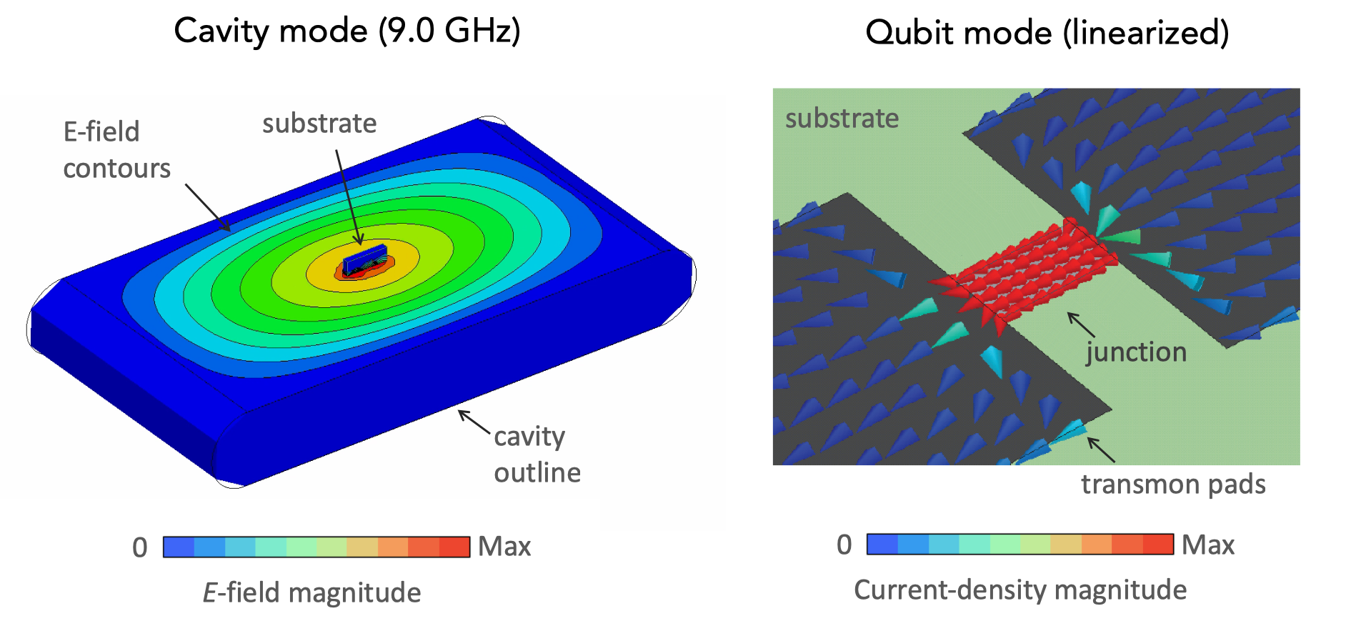
pyEPR bridges classical EM simulation and quantum circuit theory via the energy-participation ratio (EPR) method. Given a 3-D HFSS eigenmode simulation — or your own frequencies and inductances — it extracts the full quantum Hamiltonian in minutes:

1. Simulate the linearized circuit in Ansys HFSS to get eigenmode frequencies and field distributions.
2. Extract energy participation ratios $p_{mj}$ and zero-point phase fluctuations $\varphi_\mathrm{zpf}^{(mj)}$ for each junction and mode.
3. Diagonalize $H = \sum_m \omega_m a_m^\dagger a_m - \sum_j E_J[\cos\hat\varphi_j - 1 + \hat\varphi_j^2/2]$ numerically to get dressed frequencies, anharmonicities, and the dispersive-shift matrix $\chi$.

Works for any number of modes and junctions. Handles strongly anharmonic circuits (fluxonium, $\varphi_\mathrm{zpf}\gtrsim 1$). No manual circuit diagram — only the 3-D geometry.

No HFSS licence? The Hamiltonian diagonalization (steps 2–3) works with any frequencies and inductances. Start with Tutorial 6 on Binder — runs in your browser, no install.

---

Install

pip install pyEPR-quantum

Requires Python 3.9–3.12. All dependencies (numpy, qutip, matplotlib, …) are installed automatically.

conda:

conda install -c conda-forge pyepr-quantum

development install:

git clone https://github.com/zlatko-minev/pyEPR.git && cd pyEPR
pip install -e ".[test]" && pytest

Quickstart — no Ansys required

Compute the transmon anharmonicity from first principles, no HFSS needed:

import numpy as np
from pyEPR.calcs.back_box_numeric import epr_numerical_diagonalization

# Standard transmon: E_J/h = 20 GHz, E_C/h = 300 MHz
# Plasma frequency f_p = sqrt(8 E_J E_C)/h ≈ 6.93 GHz
freqs   = np.array([6.928])     # GHz  (linearised plasma frequency)
Ljs     = np.array([8.2e-9])    # H    (Josephson inductance L_J = (Phi_0/2pi)^2 / E_J)
phi_zpf = np.array([[0.416]])   # dimensionless  (n_modes x n_junctions)

# Diagonalize — returns dressed frequencies in Hz and chi matrix in MHz
f_dressed, chi_matrix = epr_numerical_diagonalization(
    freqs, Ljs, phi_zpf, cos_trunc=8, fock_trunc=15
)
print(f"Qubit frequency : {f_dressed[0].real / 1e9:.3f} GHz")
print(f"Anharmonicity   : {chi_matrix[0,0].real:.0f} MHz")
# -> Qubit frequency : 6.615 GHz
# -> Anharmonicity   : 335 MHz

For multi-mode systems, fluxonium, or custom potentials: Tutorial 6.

Full HFSS workflow

import pyEPR as epr

# 1. Connect to Ansys HFSS
pinfo = epr.ProjectInfo(project_path=r'C:\sim_folder',
                        project_name=r'cavity_with_two_qubits',
                        design_name=r'Alice_Bob')

# 2. Specify Josephson junctions
pinfo.junctions['jAlice'] = {'Lj_variable':'Lj_alice', 'rect':'rect_alice',
                              'line': 'line_alice', 'Cj_variable':'Cj_alice'}
pinfo.junctions['jBob']   = {'Lj_variable':'Lj_bob',   'rect':'rect_bob',
                              'line': 'line_bob',   'Cj_variable':'Cj_bob'}
pinfo.validate_junction_info()

# 3. Extract EPR participation ratios
eprd = epr.DistributedAnalysis(pinfo)
eprd.do_EPR_analysis()

# 4. Quantum Hamiltonian — dressed frequencies and chi matrix
epra = epr.QuantumAnalysis(eprd.data_filename)
epra.analyze_all_variations(cos_trunc=8, fock_trunc=15)
epra.plot_hamiltonian_results(swp_variable='Lj_alice')

Documentation

Full docs, API reference, and guides: pyepr-docs.readthedocs.io

Tutorial Notebooks

The tutorials are Jupyter notebooks in _tutorial_notebooks/.

#	Title	HFSS?	Topics
1	Startup example	Yes	End-to-end workflow: HFSS → EPR → χ matrix
2	Dielectric loss EPR	Yes	Dielectric energy participation, loss rates, HFSS fields calculator
3	Circuit QED parameters	No	E_J, E_C, L_J, I_c conversions; transmon model
4	Parametric sweeps	Yes	HFSS Optimetrics: linear, log, file-based sweeps
5	Generic junction potential & fluxonium	No	Exact cosine for fluxonium; custom V(phi); asymmetric SQUIDs
6	EPR without HFSS	No	Numerical workflow: supply freqs, Ljs, phi_zpf directly

Tutorials 3, 5, and 6 require only pip install pyEPR-quantum — no Ansys licence.

Video Tutorials

Tutorial 1 - Overview	Tutorial 2 - Setup of Conda & Git	Tutorial 3 - Setup of Packages & Config

Who uses pyEPR?

pyEPR is used by superconducting qubit research groups worldwide, including:

• Yale University — Michel Devoret QLab and Rob Schoelkopf RSL
• IBM Quantum and Qiskit Metal
• QUANTIC — INRIA/ENS/MINES Paris/UPMC/CNRS (Zaki Leghtas group), France
• Quantum Circuit Group — Benjamin Huard, ENS Lyon, France
• Emanuel Flurin, CEA Saclay, France
• Ioan Pop group, KIT Physikalisches Institut, Germany
• UC Berkeley, Quantum Nanoelectronics Laboratory, Irfan Siddiqi
• Quantum Circuits, Inc. · Seeqc · Alice&Bob, France · Bleximo
• Serge Rosenblum Lab, Weizmann Institute, Israel
• University of Oxford — Leek Lab
• Britton Plourde Lab, Syracuse University
• Javad Shabani Lab, NYU
• UChicago Dave Schuster Lab · Lawrence Berkeley National Lab · Colorado School of Mines
• IPQC, SJTU, Shanghai · Bhabha Atomic Research Centre, India
• Quantum Device Lab ETHZ — Andreas Wallraff · Centre for Quantum Technologies / Qcrew
• SQC lab — Shay Hacohen-Gourgy, Israel · Quantum Computing UK
• ... and many more — e-mail zlatko.minev@aya.yale.edu to be added.

Platform support

Feature	Windows	macOS	Linux
EPR / quantum analysis	Yes	Yes	Yes
Ansys HFSS COM interface	Yes	limited	limited

The HFSS COM interface uses pythoncom/win32com (Windows). On macOS/Linux you can connect to a remote Windows HFSS instance via network COM.

PyAEDT is Ansys's official cross-platform AEDT scripting library. pyEPR and PyAEDT are complementary — use PyAEDT for geometry/mesh/solve automation, pyEPR for EPR quantization.

HFSS Project Setup

Eigenmode Design — Junction setup

The EPR method requires each Josephson junction to be modelled as a lumped RLC boundary on a rectangle in HFSS, together with a polyline defining the current direction. Steps:

1. Create a rectangle for each junction (e.g., rect_alice). Assign a Lumped RLC boundary with inductance variable Lj_alice.
2. Draw a polyline spanning the junction rectangle to define current flow (e.g., line_alice).
3. The linearised Josephson inductance used in HFSS is $L_J = (\Phi_0/2\pi)^2/E_J$. The full cosine potential is restored in the quantum Hamiltonian step.
4. Enable Save Fields for each variation if running parametric sweeps (Tutorial 4).
5. Use Mixed Order solutions for best accuracy.

For a full walkthrough, see Tutorial 1 and the HFSS setup guide in the docs.

Troubleshooting

See the troubleshooting guide in the docs.

Common issues:

• pint error system='mks' unknown — upgrade pint: pip install pint --upgrade
• QuTiP not found — it is installed automatically with pyEPR-quantum; for manual install: pip install qutip
• COM Error on opening HFSS — check file path (no apostrophes/special chars); check HFSS hasn't popped an error dialog
• Parametric sweep missing field solutions — enable "Save Fields and Mesh" in ParametricSetup → Properties → Options (see Tutorial 4)
• ValueError: cannot set WRITEABLE flag — upgrade numpy

Citation

If you use pyEPR in your research, please cite:

EPR method (primary reference):

Z. K. Minev, Z. Leghtas, S. O. Mundhada, L. Christakis, I. M. Pop, M. H. Devoret, Energy-participation quantization of Josephson circuits, npj Quantum Information 7, 131 (2021) · arXiv:2010.00620

Software (Zenodo DOI for the specific version):

BibTeX for both: pyEPR.bib

Related:

• Z. K. Minev, Ph.D. Dissertation, Yale (2018), Ch. 4 — arXiv:1902.10355
• A. Petrescu, C. T. Hann, Z. K. Minev et al., EPR for very anharmonic circuits — arXiv:2411.15039

Authors and Contributors

• Authors: Zlatko Minev & Zaki Leghtas, 2015–present.
• Contributors: Phil Reinhold, Lysander Christakis, Devin Cody, Zachary Parrott, Asaf Diringer, and many others.
• Original pyHFSS.py and pyNumericalDiagonalization.py by Phil Reinhold — original repo.
• To contribute: open a GitHub issue or PR, or contact Z. Minev.